Objective of VAE
- Compute the posterior $p_\theta(z|x)$ which takes data from observation to latent space
- $\textcolor{red}{p_\theta(z|x)} p_\theta(x) = p_\theta(x,z)$ is the expression for this term!
- LHS: first term we want to find! second term we can’t find!
- RHS: gives us the chance of having (observation, latent) pair, describes everything!
- $\textcolor{red}{p_\theta(z|x)} p_\theta(x) = p_\theta(x,z)$ is the expression for this term!
- $p_\theta(x) = p(x;\theta)$ = evidence = marginal likelihood = true distribution parameterised by $\theta$
- Maximise the evidence $p_\theta(x)$ ⇒ MLE on the true data distribution!
💡 Both depend on us evaluating the evidence/marginal likelihood $p_\theta(x)$, whose calculation is intractable. Why? We can try to find evidence by integrating latent variables $z$:
- $p_\theta(x) = \int p_\theta(x|z)p(z) \ dz = \int p_\theta(x,z)\ dz$, require us to integrate over the latent variable, which usually is in a high dimension and can take a large range of values!
- This makes calculation impossible / intractable!
KL-Divergence
- Measures the divergence between two distributions
- Inspired from the difference between log-likelihood (AKA log likelihood ratio)
- $\log \frac{p_\theta(x)}{q_\theta(x)}$ and we take the mean of this:
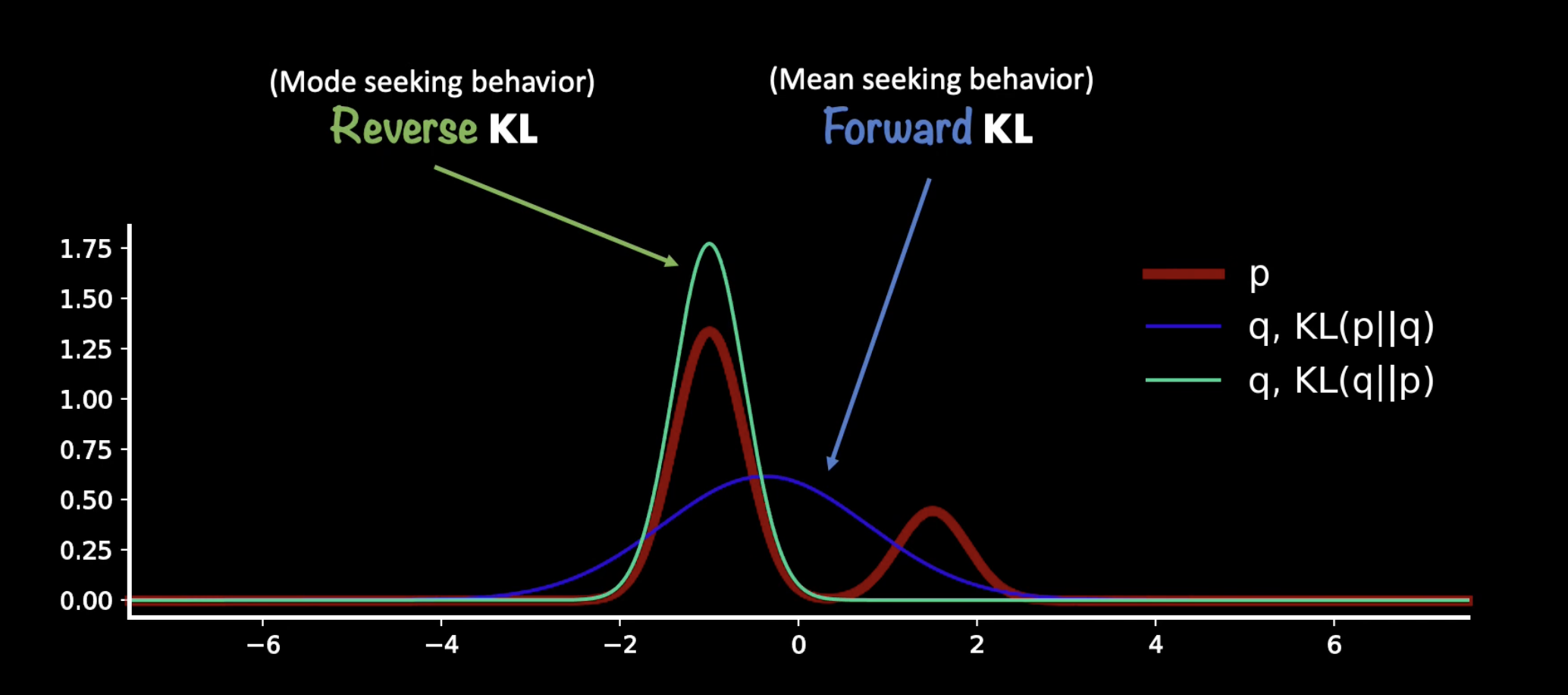
💡 Notice that the expectation is taken WRT $p_\theta$, the numerator ⇒ this is called forward KL
There are forward, $D_{KL}(p_\theta||q_\phi)$ and reverse, $D_{KL}(q_\phi||p_\theta)$ divergence which gives different optimising result for learnt distribution q:
Evidence Lower Bound (ELBO)
This method allows us to model the evidence ( denominator of the Baye’s theorem, $p_\theta(x)$ ) with another analysable distribution $q_\phi(x)$.
Therefore we can also approximate the posterior distribution (encoder) with another distribution that is computable, $q_\phi(z|x)$. We will use optimisation techniques to find the computable variable.
^We assume this can be learnt by the neural network!
The KL definition gives us some meaningful relationships: we can manipulate the equation to find how to best conform to the true distribution using the approximated distribution.
Simplifying this KL term:
$$ D_{KL}(\ q_\phi(z|x) \ || \ p_\theta(z|x)\ ) = E_{z \sim q_\phi(z|x)}[\log q_\phi(z|x)] - E_{z \sim q_\phi(z|x)}[\log p_\theta(z|x)] $$ $$ D_{KL}(\ q_\phi(z|x) \ || \ p_\theta(z|x)\ ) = E_{z \sim q_\phi(z|x)}[\log q_\phi(z|x)] - E_{z \sim q_\phi(z|x)}[\log p_\theta(z,x) - \log p_\theta(x)] $$Note the independence between p and q, hence:
$$ D_{KL}(\ q_\phi(z|x) \ || \ p_\theta(z|x)\ ) = E_{z \sim q_\phi(z|x)}[\log q_\phi(z|x)] - E_{z \sim q_\phi(z|x)}[\log p_\theta(z,x)] + \log p_\theta(x) $$As KL-divergence (LHS) is always non-negative, the evidence lower bound is therefore:
$$ \log p_\theta(x) \geq \textcolor{red}{L_{\text{ELB}}} = - E_{z \sim q_\phi(z|x)}[\log q_\phi(z|x)] + E_{z \sim q_\phi(z|x)}[\log p_\theta(z,x)] $$This already gives us an equation that allow us to maximise the likelihood. Now, we examine and dissect the equation further to try to understand it:
$$ L_{\text{ELB}} = - E_{q_\phi}[\log q_\phi(z|x)] + E_{q_\phi}[\log p_\theta(z|x) + \log p_\theta(x)] $$ $$ L_{\text{ELB}} = E_{q_\phi}[\log p_\theta(x)- \log q_\phi(z|x)] + E_{q_\phi}[\log p_\theta(x|z)] $$Note that the first term would be a reverse KL, but we can apply negation to get the forward KL:
$$ \color{blue} L_{\text{ELB}} = -D_{KL}(\ q_\phi(z|x) \ || \ p_\theta(x)\ )+ E_{z \sim q_\phi(z|x)}[\log p_\theta(x|z)] $$We want to maximise ELBO, which consists of:
minimise the negated KL term: how similar the posterior is to the prior
Effectively, this regularises the complexity of latent space
we usually set the prior to be standard normal distribution, which allow us to get a closed form equation:

maximise the likelihood: how likely to see the observation given this latent
$$ E_{z \sim q_\phi(z|x)}[\log p_\theta(x|z)] \approx \frac{1}{N} \sum_{i=1}^{N} {q_\phi(z_i|x)}\log p_\theta(x|z_i) $$Average over the latent variables (approximated by taking N samples from the encoding distribution)
Intuitively, this is the same as taking samples of z = mu * zeta + epsilon (sampled from the learnt encoding function), and calculating the average of the log likelihood
Under the assumption of $q$ being a normal distribution, we can use the property that likelihood = MSE + constant
By minimising the negated ELBO, we are doing two things:
- we minimises the KL-divergence term ⇒ we want posterior distribution to be close to prior
- we minimises the negative log-likelihood ⇒ we want reconstructed x to be similar to x
💡 The reconstruction error can be interpreted as equivalent to negative log-likelihood.
Maximizing the likelihood of the observed data under the generative model is equivalent to minimizing the negative log-likelihood. Minimizing the negative log-likelihood encourages the model to generate data that closely matches the observed data.
“Duality” view
Taking the duality view, since:
$\log p_\theta(x) = L_{ELB} + D_{KL}(\ q_\phi(z|x) \ || \ p_\theta(z|x)\ )$
If we are maximising $L_{ELB}$, we are also making sure we are minimising $D_{KL}(\ q_\phi(z|x) \ || \ p_\theta(z|x)\ )$
Which is trying to “match” the approximate distribution to the underlying true distribution!
Reference
A Tutorial on Variational Autoencoders with a Concise Keras Implementation | Louis Tiao
Variational Autoencoder: Intuition and Implementation - Agustinus Kristiadi
